Outline
Note: DATTES 22.06 example. Do not work with DATTES 23.05.
Information about the dataset
The center for advanced life cycle engineering (CALCE) provides open access to experimental test data on lithium-ion batteries, which includes continuous full and partial cycling, storage, dynamic driving profiles, open circuit voltage measurements, and impedance measurements.
These dataset have been used in CALCE publications listed here. For the full details of the study and data reuse conditions, please refer to their website
Information about the test
In this example, the test over the cylindrical cell INR18650-20R will be analyzed. The methology can be followed for any of the data provided by CALCE.
The test is a characterization test realised with a Arbin BT2000 battery cycler over fresh SAMSUNG SDI INR 18650-20R.
Data analysis with DATTES
Low Current OCV-Initial Capacity Data
In this example, it is assumed that DATTES is installed on your computer. If it is not the case, please follow these instructions : Getting started.
- First, DATTES must be initialized
% Change the working folder to reach DATTES repository
cd DATTES_folder
% Initialize DATTES
initpath_dattes
- Then, change the working folder to reach CALCE data.
% Change the working folder to reach experimental data
cd CALCE_databank
- Convert the Arbin result files into .xml format
% Convert the Arbin .xls result files in current folder ('.') into .xml format
arbin_xls2xml('.')
- Gather all xml files into a single variable
% Search for .xml files in current folder ('./')
XML_list=lsFiles('.','.xml')
- Load the configuration (‘cvs’ = configure + verbose + save)
[result]=dattes(XML_list,'cvs','cfg_SAMSUNG_INR18650_20R_2Ah')`
- Plot configuration (‘Gc’ = Graphics + configuration):
[result]=dattes(XML_list,'Gc')
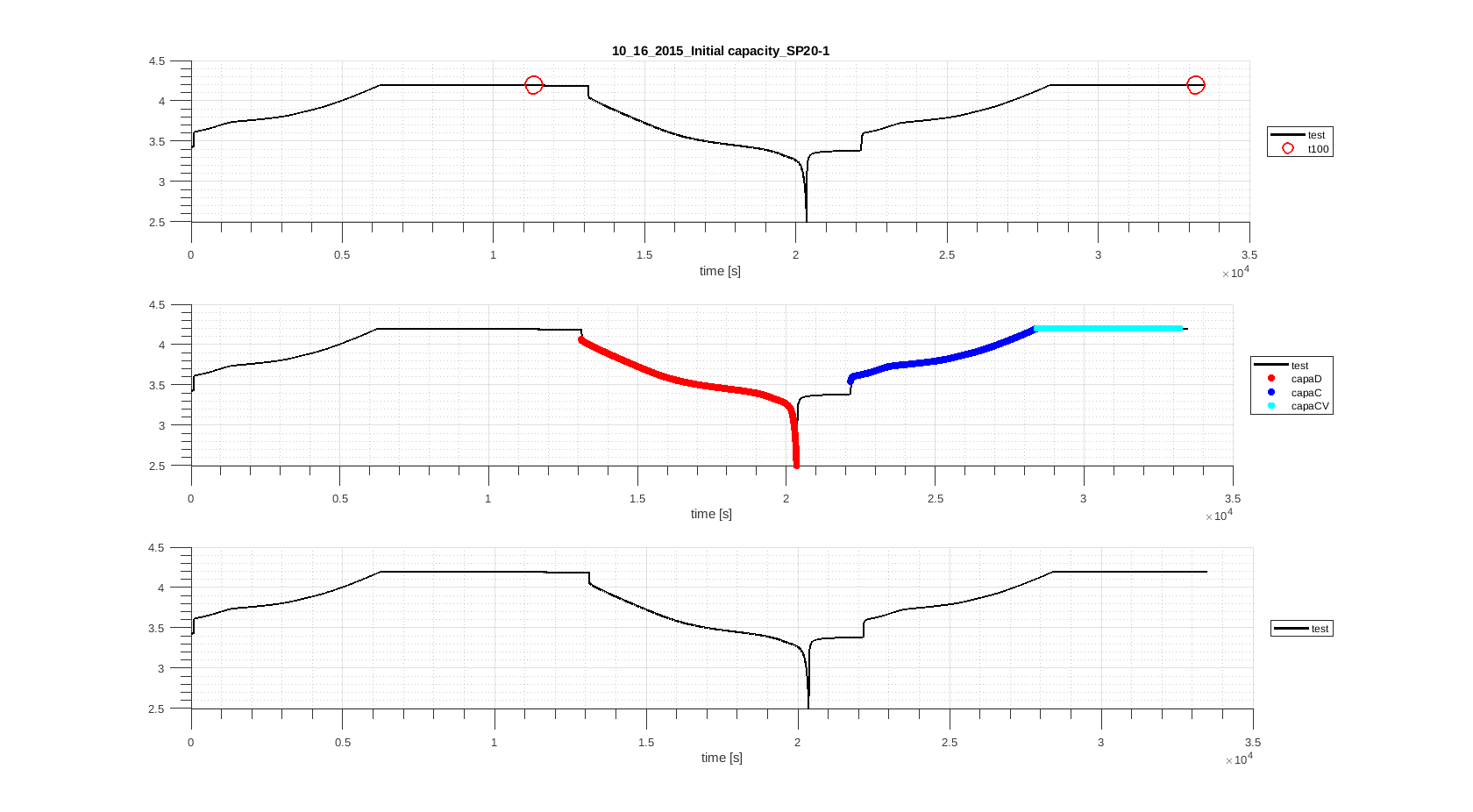
First subplot shows cell voltage (black line) and moments when DATTES identified full charges (SoC100 reference). Second subplot show which phases have been identified by DATTES for capacity measurement: red = full CC discharge; blue = full charge (CC part); cyan = ful charge (CV part).
- Plot phases (‘Gp’ = Graphics + pĥases):
[result]=dattes(XML_list,'Gp')
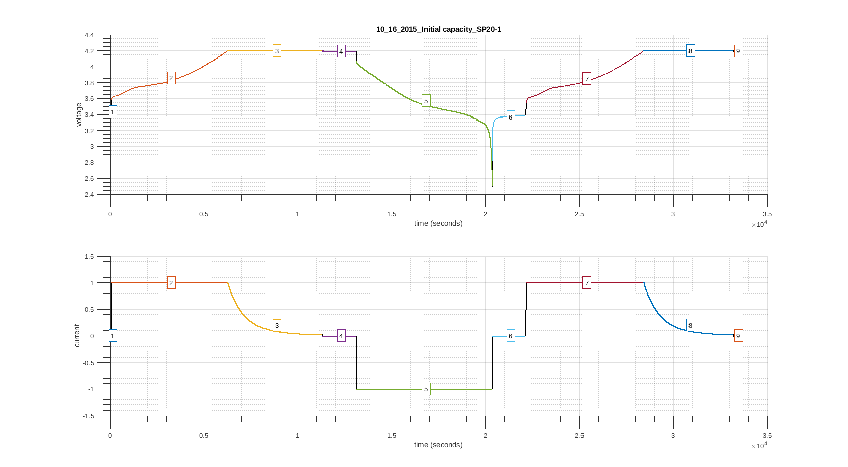
This plot show differents phases identified by DATTES (cut into phases depending of cycler working mode: CC, CV, rest, etc.).
- Calculate the capacity and the soc (‘CSvs’ = Capacity + SoC + verbose + save’):
[result]=dattes(XML_list,'CSvs')
- Plot capacity (‘GC’ = Graphics + capacity):
[result]=dattes(XML_list,'GC')
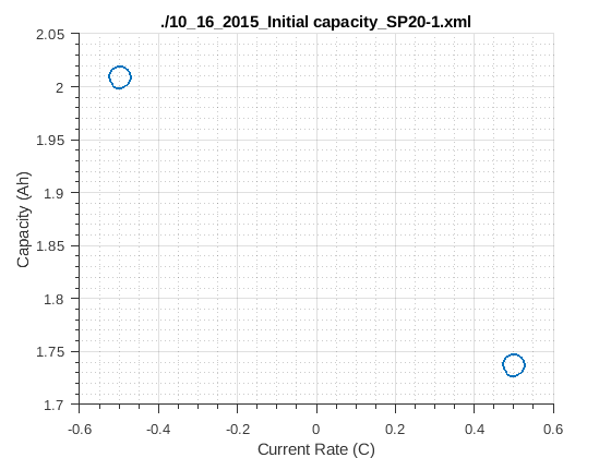
This plot shows capacity values for CC discharge and for CC charge identified precedently versus current rate (-0.5C for discharge, 0.5C for charge).
- Plot state of charge (‘GS’ = Graphics + SoC):
[result]=dattes(XML_list,'GS')
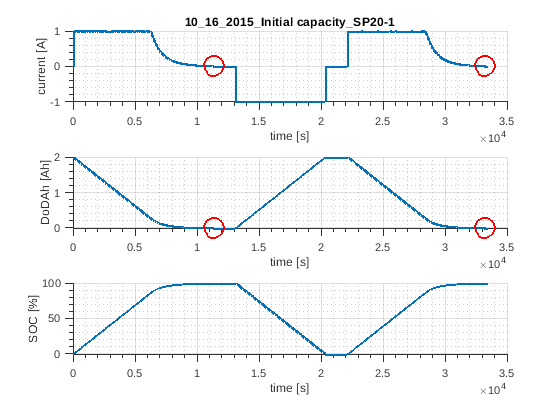
These three subplots show current profile (A), depth of discharge (Ah) and SoC (%) during the test. Red circles correspond to full charge moments identified by DATTES (SoC100 reference).
Low Current OCV-Data
In this example, it is assumed that DATTES is installed on your computer. If it is not the case, please follow these instructions : Getting started.
The low current ocv at 0°C data file is analysed : Link
- First, DATTES must be initialized
% Change the working folder to reach DATTES repository
cd DATTES_folder
% Initialize DATTES
initpath_dattes
- Then, change the working folder to reach CALCE data.
% Change the working folder to reach experimental data
cd CALCE_databank
Note : CALCE file format
CALCE data files have been generated by Arbin cycler under a .xls format. The preferable format may have been .xlsx as the Microsoft Excel used to generate data was a Microsoft Excel 2007+.
To process CALCE data with DATTES it is necessary to change the change the files extension to .xlsx
- Change result files format to .xlsx
% Change result files extension to .xlsx
! mv 02_24_2016_SP20-1_0C_lowcurrentOCV.xls 02_24_2016_SP20-1_0C_lowcurrentOCV.xlsx
- Convert the Arbin result files into .xml format
% Convert the Arbin .xls result files in current folder ('.') into .xml format
arbin_xls2xml('.')
- Gather all xml files into a single variable
% Search for .xml files in current folder ('./')
XML_list=lsFiles('.','.xml')
- Load the configuration (‘cvs’ = configure + verbose + save)
[result]=dattes(XML_list,'cvs','cfg_SAMSUNG_INR18650_20R_2Ah')`
- Plot configuration (‘Gc’ = Graphics + configuration):
[result]=dattes(XML_list,'Gc')
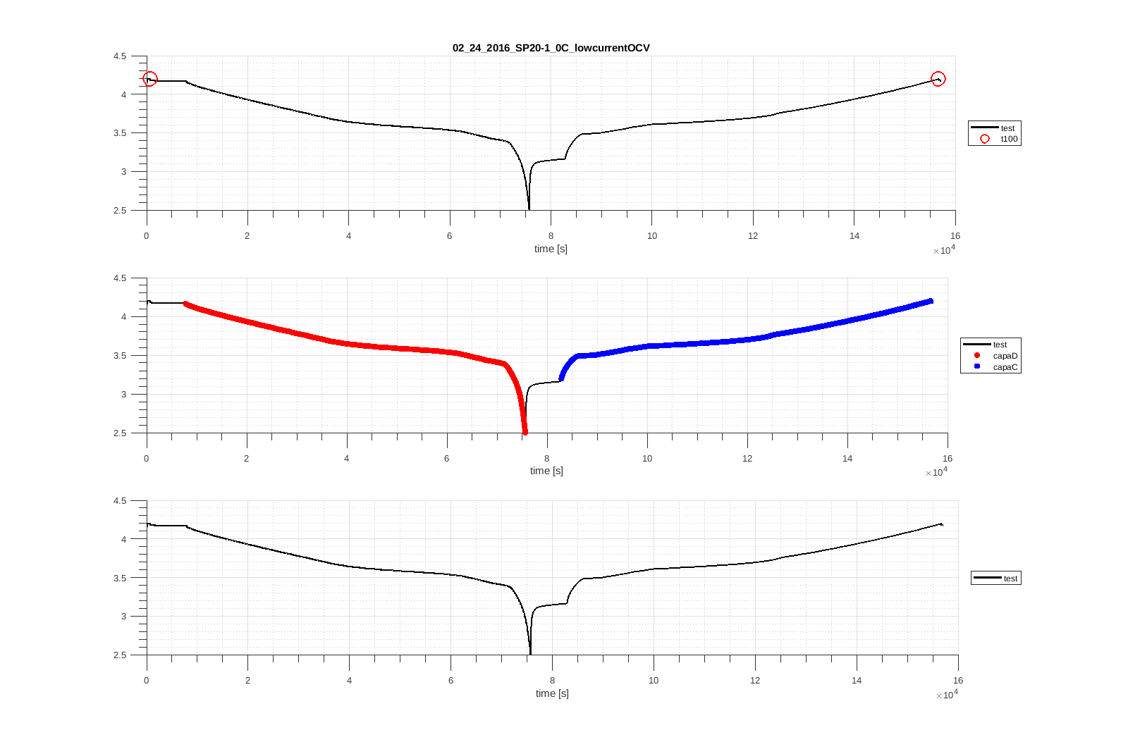
First subplot shows cell voltage (black line) and moments when DATTES identified full charges (SoC100 reference). Second subplot show which phases have been identified by DATTES for capacity measurement: red = full CC discharge; blue = full charge (CC part); cyan = ful charge (CV part).
- Plot phases (‘Gp’ = Graphics + phases):
[result]=dattes(XML_list,'Gp')
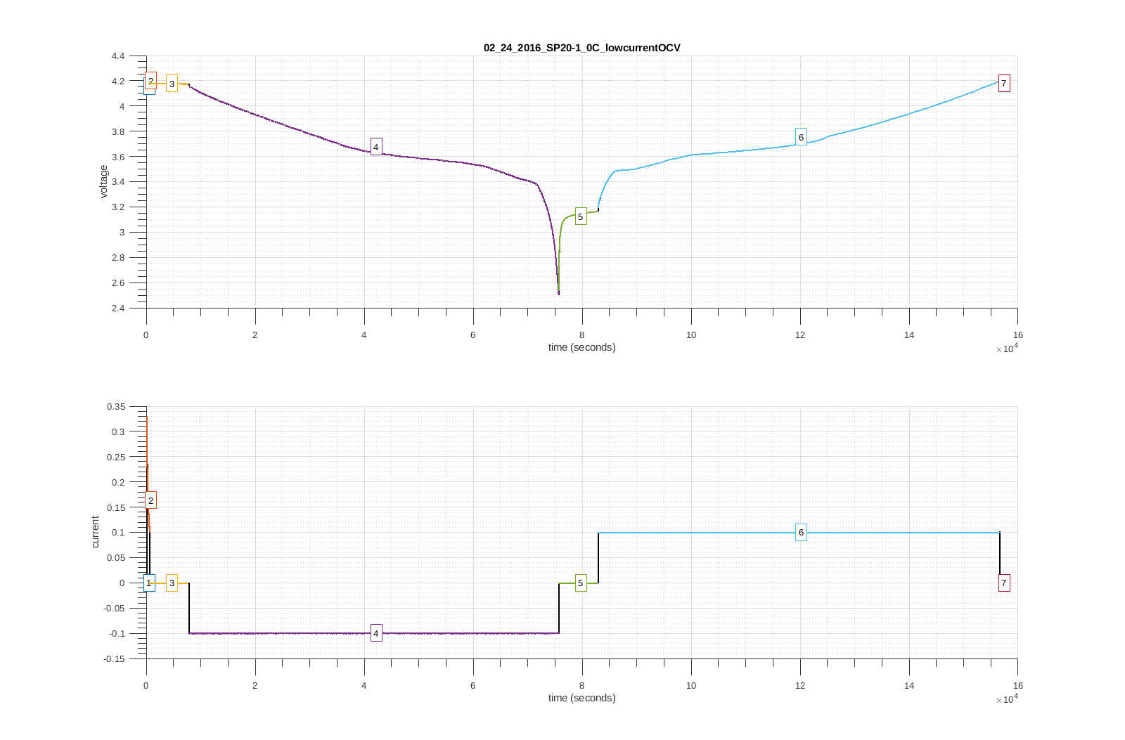
This plot show differents phases identified by DATTES (cut into phases depending of cycler working mode: CC, CV, rest, etc.).
- Calculate the capacity and the soc (‘CSvs’ = Capacity + SoC + verbose + save’):
[result]=dattes(XML_list,'CSvs')
- Plot capacity (‘GC’ = Graphics + capacity):
[result]=dattes(XML_list,'GC')
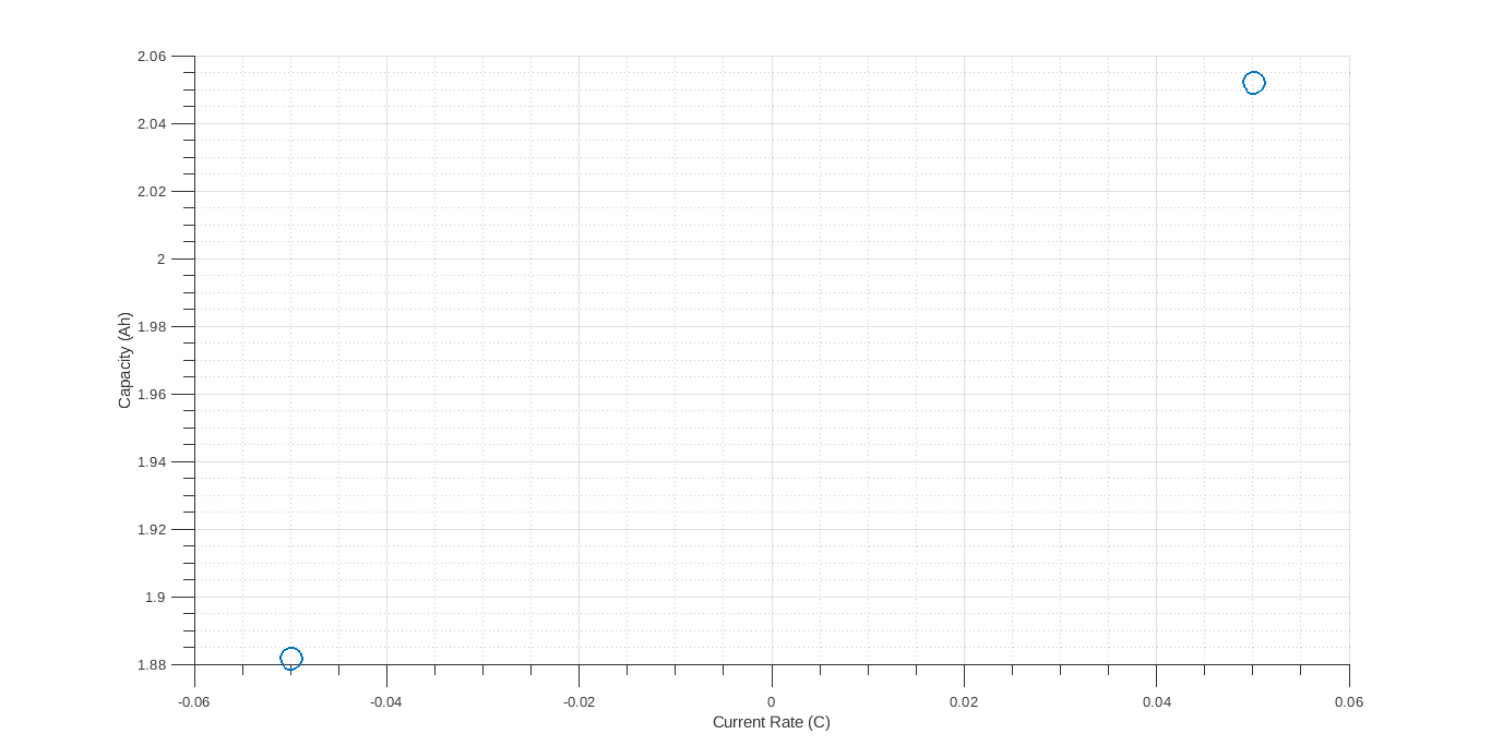
This plot shows capacity values for CC discharge and for CC charge identified precedently versus current rate (-0.05C for discharge, 0.05C for charge).
- Plot state of charge (‘GS’ = Graphics + SoC):
[result]=dattes(XML_list,'GS')
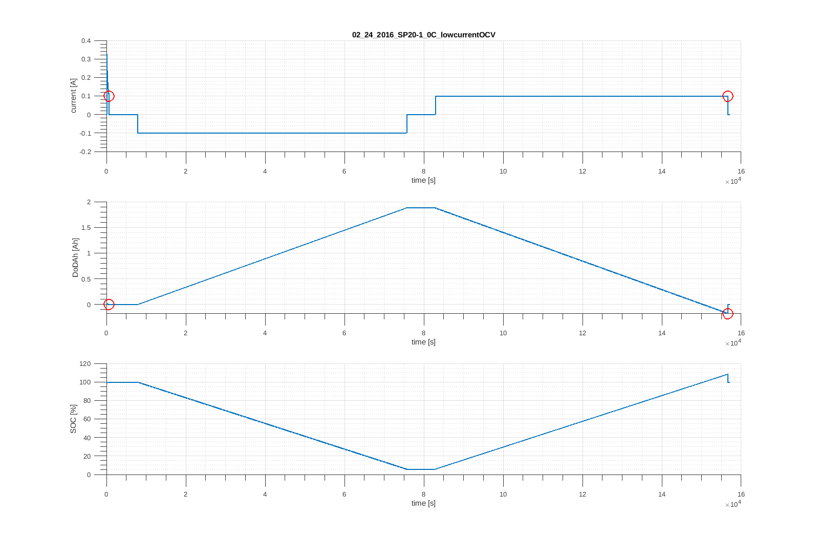
These three subplots show current profile (A), depth of discharge (Ah) and SoC (%) during the test. Red circles correspond to full charge moments identified by DATTES (SoC100 reference).
- Calculate the pseudo OCV (‘Pvs’ = pseudo OCV + verbose + save’):
[result]=dattes(XML_list,'Pvs')
- Plot pseudo OCV (‘GP’ = Graphics + pseudo OCV):
[result]=dattes(XML_list,'GP')
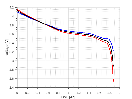
This plot shows pseudo OCV for discharge, CC charge and for average between charge and discharge.
- Plot efficiency (‘GE’ = Graphics + efficiency):
[result]=dattes(XML_list,'GE')
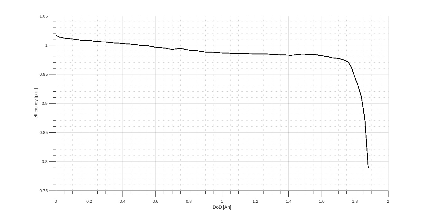
This plot shows pseudo OCV for discharge, CC charge and for average between charge and discharge.
- Analyse the incremental capacity analysis (‘Ivs’ = ICA + verbose + save’):
[result]=dattes(XML_list,'Ivs')
- Plot ICA, DVA and OCV (‘GI’ = Graphics +ICA +DVA + OCV ):
[result]=dattes(XML_list,'GI')
