Outline
- Capacity definition
- Analysis preparation
- Anomaly detection
- Capacity analysis
- Result visualization
- Methodology and hypothesis
- Contribute to capacity analysis
Capacity definition
The capacity is the quantity of charges that a battery can store or deliver at a given current rate. It is calculated by integrating the current charged or discharged between the minimal and maximal voltage of the battery.
In charge $$ Q= \int_ \mathrm{t_{Umin}}^\mathrm{t_{Umax}} \mathrm{i(t)} \mathrm{d}t$$
In discharge $$ Q= \int_ \mathrm{t_{Umax}}^\mathrm{t_{Umin}} \mathrm{i(t)} \mathrm{d}t$$
with
- Q : the rated capacity (Ah)
- i(t) : the current (A)
- tUmax : the instant at which cell voltage is maximum (s)
- tUmin : the instant at which cell voltage is minimum (s)
Capacity is usually measured by making a sequence of full charge and discharge in constant current - constant voltage mode. As an example, in charge the battery is fully charged with a constant current until the maximal voltage is reached. Then, voltage is maintained at this upper limit by reducing the current until it reach a threshold value. The definition of the voltage threshold depends on the battery chemistry and the recommendations given by the manufacturer.
Analysis preparation
DATTES is called as follows : [result]=dattes(XML_file,'action','configuration_file').
Before any analysis, it is then necessary to create the XML and configuration files.
The section Import cycler files explains how to create the XML file.
The section Create a configuration file explains how to create a configuration file.
Anomaly detection
Capacity tests may be affected by abnormally long constant voltage step and noise.
To check if a capacity test have run normally the action ‘c’ should be used :
[result] = dattes(XMLfile,'cvs'); and plotted : [result] = dattes(XMLfile,'Gc');
A normal capacity test should look like the following image :
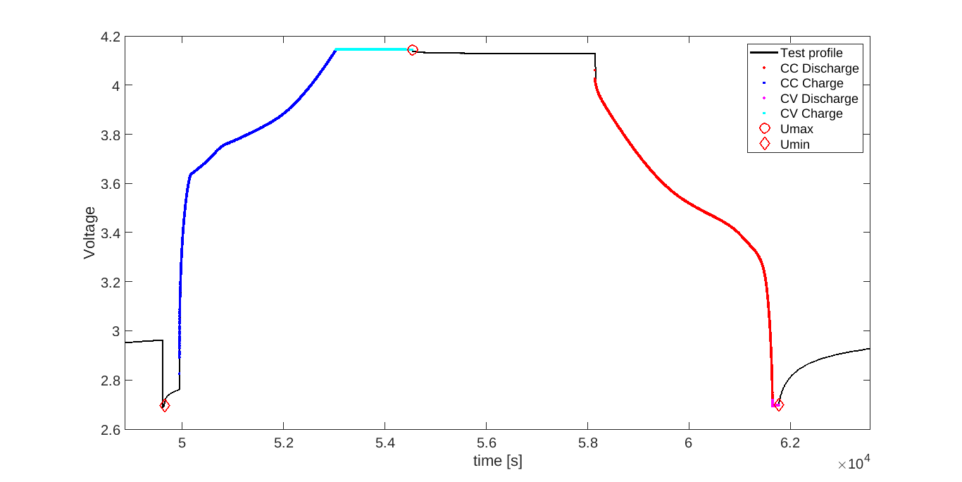
Anomaly can be easily identified if one of the following elements is not detected :
- CC discharge phase
- CC charge phase
- CV discharge phase
- CV charge phase
- Umax threshold
- Umin threshold
Capacity analysis
To analyze the capacity, the action ‘C’ should be used :
[result] = dattes(XMLfile,'Cvs');
The output are :
| Output structure | Field | Array | Unit | Description |
|---|---|---|---|---|
| result | capacity | cc_capacity |
Ah | Capacity measured during the constant current phase |
| result | capacity | cc_crate |
- | Current rate during the constant current phase |
| result | capacity | cc_time |
s | Instant of the beginning of the constant current phase |
| result | capacity | cc_duration |
s | Duration of the constant current phase |
| result | capacity | cv_capacity |
Ah | Capacity measured during the constant voltage phase |
| result | capacity | cv_crate |
- | Current rate during the constant voltage phase |
| result | capacity | cv_time |
s | Instant of the beginning of the constant voltage phase |
| result | capacity | cv_duration |
s | Duration of the constant voltage phase |
| result | capacity | cc_cv_time |
s | Final time of cc part of each CC-CV capacity measurement |
| result | capacity | cc_cv_capacity |
Ah | Sum of CC and CV capacity measurements |
| result | capacity | cc_cv_duration |
s | Sum of CC and CV capacity durations |
| result | capacity | cccv_ratio_cc_ah |
Ah | CC / CV part of capacity measurements |
| result | capacity | cccv_ratio_cc_duration |
s | Duration of CC / CV part of capacity measurements |
Result visualization
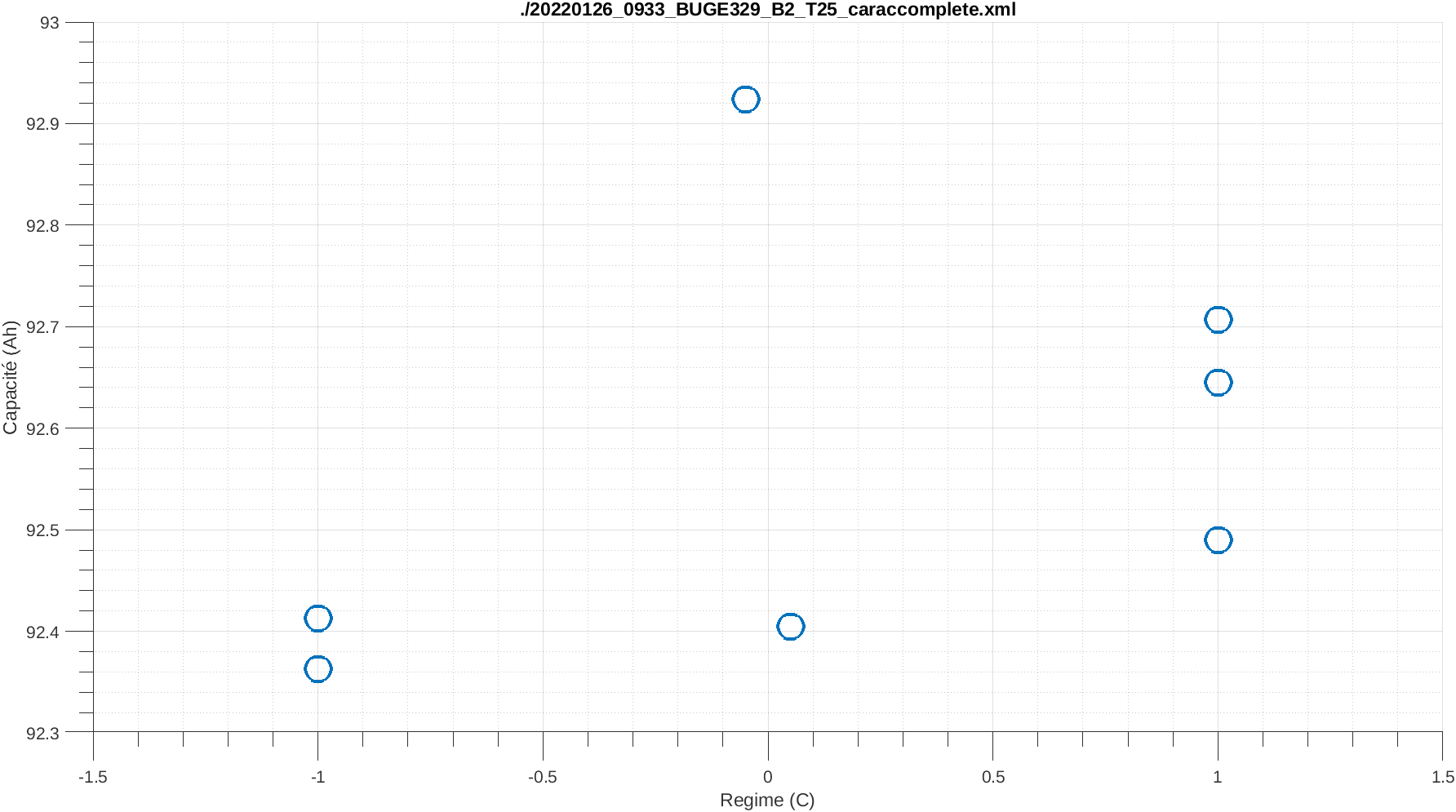
To visualize the capacity, the action ‘GC’ should be used :
[result] = dattes(XMLfile,'GC');
The graph should look like
Methodology and Hypothesis
Method
The capacity is calculated by summing the capacity calculated during the DC phase with that of a possible CV phase.
The capacity is calculated by the ident_capacity function with the following code:
%CC part
Capa = abs([phases(config.pCapaD | config.pCapaC).capacity]);
Regime = [phases(config.pCapaD | config.pCapaC).Iavg]./config.Capa;

%CV part
phasesCV = phases(config.pCapaDV | config.pCapaCV);
CapaCV = abs([phases(config.pCapaDV | config.pCapaCV).capacity]);
dCV = [phasesCV.duration];
UCV = [phasesCV.Uavg];
Key parameters for the calculation
The four key parameters for the calculation of the capacity are :
- config.pCapaD,
- config.pCapaC,
- config.pCapaDV,
- config.pCapaCV.
They are determined in configurator :
%1) phases capa decharge (CC):
%1.1. imoy<0
%1.2 - end at SoC0 (I0cc)
%1.3 - are preceded by a rest phase at SoC100 (I100r or I100ccr)
pCapaD = [phases.Imoy]<0 & ismember(tFins,t(I0cc)) & [0 pRepos100(1:end-1)];
%2) phases capa charge (CC):
%2.1.- Imoy>0
%2.2 - end at SoC100 (I100cc)
%2.3 - are preceded by a rest phase at SoC0 (I0r or I0ccr)
pCapaC = [phases.Imoy]>0 & ismember(tFins,t(I100cc)) & [0 pRepos0(1:end-1)];
% pCapaC = [phases.Imoy]>0 & [0 pRepos0(1:end-1)];%LYP, BRICOLE
%3) residual load phases
%1.1.- Imoy<0
%1.2 - end at SoC0 (I0)
%1.3 - are preceded by a phase pCapaD
pCapaDV = [phases.Imoy]<0 & ismember(tFins,t(I0)) & [0 pCapaD(1:end-1)];
%4) residual load phases
%1.1 - Imoy>0
%1.2 - end at SoC100 (I100)
%1.3 - are preceded by a phase pCapaC
pCapaCV = [phases.Imoy]>0 & ismember(tFins,t(I100)) & [0 pCapaC(1:end-1)];
Assumptions and possible simplifications
A trapezoidal rule have been preferred for the calculation of Ah:
Contribute to capacity analysis
A list of open issues related to capacity calculation and visualization may be available here.